Programming is just implementing complex calculations, right? I naively assumed so, but when I embarked upon the data scientists’ journey, the data began to balloon; and so did the fundamental challenges that sneak by the naive developer. When data gets big, one naturally hits constraints, and it beckons a more elaborate perspective and toolset. Inevitably, the developer descends into the different layers of the Inferno.

Initially, she will come across the limitations of memory. Computers have various means of storing memory. The most prominent are hardware storage (files on a drive) – similar to durable, etched stone - or random access memory (RAM) - memory easily graspable, but ephemeral. Consume too much RAM and the operating system freezes; output too much data/too many files and hard drives crash. There are also intricate problems to each memory type: computation overhead is associated with drive storage, but RAM per gigabyte is much more expensive than drive storage. In scientific computing, the data can consume so many resources that one has to cleverly negotiate her options on how to store and manipulate data. The primary way to reduce memory constraints is to think about what data is pertinent, and what structures the data are stored in – a programmer has a toolbelt of different data structures, but not all data structures use memory equally and it’s thus important to use the right hammer for the job. Second, the developer must negotiate between what is hogging memory, what is pertinent to store in RAM and what can be offloaded to the drive(s). Again, the program incurs the overhead of input/output (I/O) operations when outputting to files, but it becomes a necessary trade-off when RAM is too expensive.

Descending further into data structures, the developer naturally encounters matrices. Matrices become an essential tool for linearizing the relationship between input size and computation time because many matrix calculations are implemented more efficiently. For example, when conducting pairwise comparisons, or comparing all inputs against all other inputs, execution time becomes a quadratic function. Computer calculations are incredibly fast, but what if the input is 100,000 proteins from 5 genomes? Now the execution has ballooned to 10,000,000,000 calculations. This prevents software scalability, making the input size more

prohibitive. Matrix-based calculations can take those pairwise comparisons and break apart the quadratic relationship. This is so useful that graphical processing units (GPUs) have been specifically designed for matrix operations – instead of reading video frames pixel by pixel in a video, GPUs can process data like an apple slicer. The downside of matrix operations is these structures can consume a lot of memory and matrix implementation is not always straight forward. Some programming languages, such as R, are built around matrix computing, so many operations developers are familiar with are already using linear algebra. Other languages, such as Python, have great package support for matrix operations, but the standard operations often are not.

Alas, some operations are just inefficient in matrices or there may not be a feasible path for implementing matrix-based equivalents. So the developer descends into the third layer – processing speed. Why not just use faster processors? Moore’s Law, which is related to processor speed, is physically limited by how small silicon transistors can be. As this asymptote has been approached, there has been an accompanying decrease in the velocity with which newer processer speeds are developed. This has led to increased emphasis on processors with multiple cores and threads through which tasks can be parallelized to execute in tandem. Instead of calculations performed 1 by 1, they are moved into n by n space. The eager developer may wish to just tell a program, “I COMMAND YOU TO RUN ON 4 CPUS!”

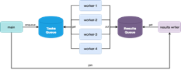
but will be disappointed when the program fails. The programs themselves have to intelligently plan distributing a task over multiple cores. From the developer standpoint, this manifests as 1) setting up a function that can be executed in parallel, 2) distributing the data over that function, and 3) recombining and parsing that data. Overhead is incurred with parallelizing operations and moving data between processors, so the data inputted into parallelized functions needs to be minimized. Furthermore, developers may need to be clever and create complex distribution techniques comprised of workers and queues with independent concurrent process functions that can read data, feed data into one another, move data to output, etc. It seems intuitive that execution speed is a function of the number of parallel processors, however the complexity of implementing parallelization breaks that relationship. In fact, there is often a limit to the efficiency increases of multiple processes; sometimes execution gets slower with more processors! Entire programming languages exist partially on the premise of making parallelization easier, and it’s one of the foremost critiques of Python.

The developer may descend deeper into learning these new languages, experimenting with different approaches. I have not touched on a different form of parallelization, threading, or other data management techniques. The point is that software development is a journey into developing a toolset and somewhat of an art in implementation. As the developer goes further, the journey is dark ahead, and I have yet to journey beyond.

Written by TPS graduate student Zach Konkel